November 2024.

When you start reading diffusion papers, you’ll quickly come across an equation like this:

$$dx = f(x,t)dt + g(x,t)dw$$

where $w$ is Brownian motion. When I first saw these, I admit that I just thought about the discretized version

$$\Delta_x = f(x,t)\Delta_t + g(x,t)\Delta_w$$

and moved on. You can generate approximate samples in code easily enough:

dt = 0.001
x_last = 0
t = 0

while t < 1:
    dw = np.random.normal(0, np.sqrt(dt))
    x_next = x_last + f(x_last,t)*dt + g(x_last,t)*dw
    
    t += dt
    x_last = x_next

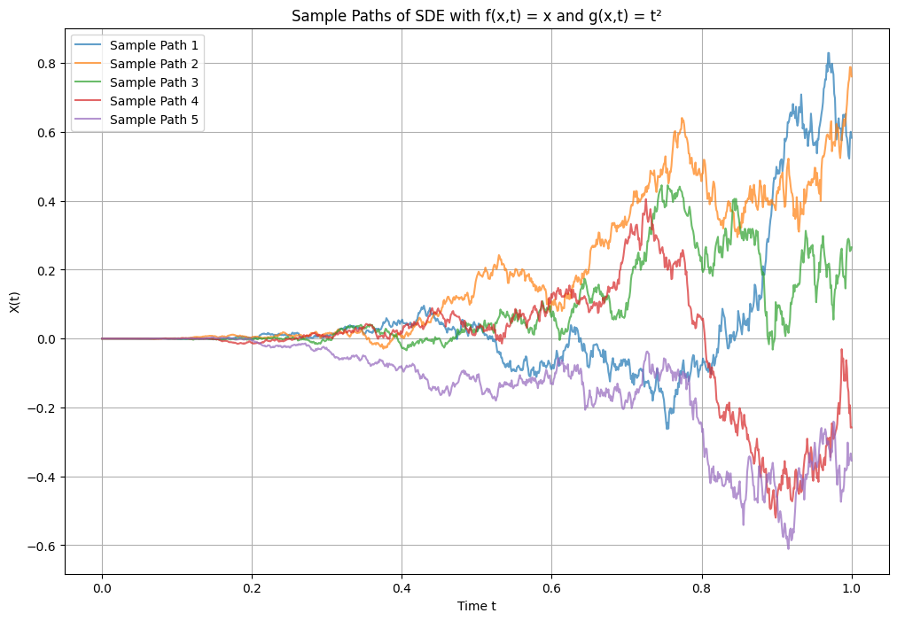
Here’s a sample plot with $f(x,t) = x$ and $g(x,t) = t^2$:

But discretization feels bad. Sir Isaac Newton didn’t brave plague, sizardom, and falling apples just so that we could discretize. Let’s have some respect. Because you do lose something when you discretize. Here’s Brownian motion at a few different resolutions, becomming more and more jagged as $dt$ becomes finer:

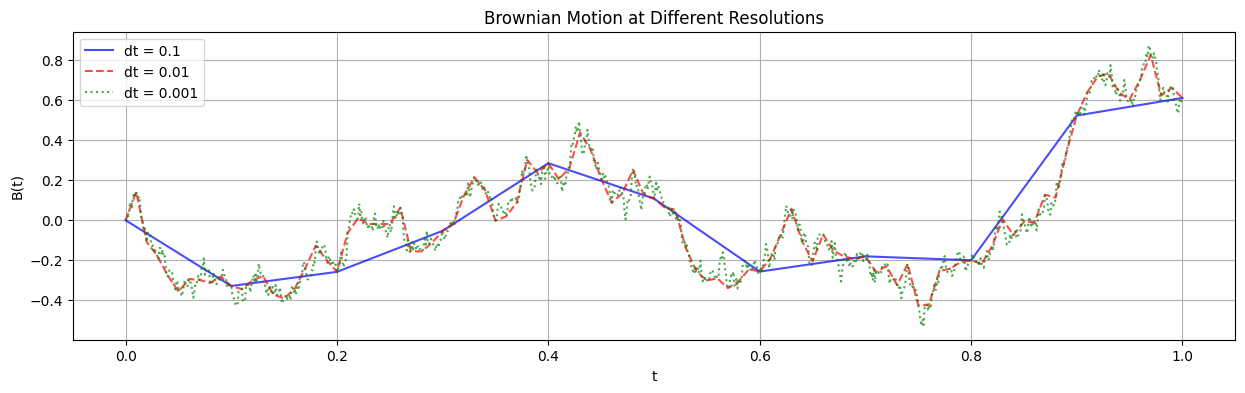
Look at that smooth-ish curve when $dt = 0.1$. That’s not honest Brownian motion. And if we zoomed in, we’d be similarly disgusted with $dt=0.01$ and $dt=0.001$. I mean, these curves are differentiable almost everywhere. We need something better, we need an infinitesimal notion of “noise”.

So what does the equation

$$dx = f(x,t)dt + g(x,t)dw$$

actually mean? What’s the real, stochastic calculus interpretation?

Stochastic Integration

One answer — and this is actually the formal answer in one school of thought — is that the “differential” equation $dx = f(x,t)dt + g(x,t)dw$ is just shorthand for an integral equation:

$$x = \int_0^T f(x,t)dt + \int_0^T g(x,t)dw.$$

Keep in mind here that $x$ and $w$ are both stochastic processes depending on $t$, so it’s probably clearer to write

$$x_t = \int_0^t f(x,s)ds + \int_0^t g(x,s)dw_s.$$

We understand the integral on the left hand side. Now we have to make sense of the integral on the right.

It’s going to be confusing to use $w$ to refer to Brownian motion given some notation that’s coming later, so let’s use $B_t$ instead. In general, we might want to integrate not just some deterministic function $g(x,t)$ but some other stochastic process $H_t$. So, in the end, we’re trying to define

$$I(t) = \int_0^t H_s dB_s$$

The rest of this post is going to be about defining & making sense of this integral.

Intuitively, what should the integral be? If we chop $[0,t]$ into a bunch of sub-intervals $[t_i, t_{i+1}]$, then by analogy to Riemann integration, we hope that the integral above will be well-approximated by

$$\sum_{i=1}^{n} H_{t_{i-1}}(B_{t_i} - B_{t_{i-1}})$$

if we make all the $[t_{i-1}, t_i]$ really small. (We’ll say that the “mesh size” goes to zero if $t_i - t_{i-1} \to 0$ for all $i$ uniformly in $i$.)

And this does in fact work. Choose some sequence $\pi_n$ of partitions of $[0,t]$ with mesh size going to zero. Define

$$\int_0^t H_s dB_s = \lim_{n\to\infty} \sum_{[t_{i-1}, t_i] \in \pi_n}^{n} H_{t_{i-1}}(B_{t_i} - B_{t_{i-1}}).$$

We have to put some regularity conditions on $H_s$ to guarantee convergence: it’s enough that $\int_0^t H_s^2ds < \infty \space \forall t$.

Done. But…

Some Surprises

Now let’s try to actually integrate something. Let’s set $H_t = B_t$, so we’re integrating

$$\int_0^t B_s dB_s.$$

For a partition $\pi_n$, we look at the sum

$$\sum_{[t_{i-1}, t_i] \in \pi_n}^{n} B_{t_{i-1}}(B_{t_i} - B_{t_{i-1}}) = \frac{1}{2}\sum (B_{t_i}^2 - B_{t_{i-1}}^2) - \frac{1}{2} \sum (B_{t_{i}}- B_{t_{i-1}})^2.$$

The first sum $\frac{1}{2}\sum (B_{t_i}^2 - B_{t_{i-1}}^2)$ telescopes, and goes to $\frac{1}{2}B_t^2$. Let’s look at the second sum. $B_{t_i} - B_{t_{i-1}}$ is a normal random variable with mean zero and variance $t_i - t_{i-1}$. So the expected value of $(B_{t_i} - B_{t_{i-1}})^2$ is $t_i - t_{i-1}.$ So the expected value of the whole sum is just $t$. By a similar argument, the variance of $B_{t_i} - B_{t_{i-1}}$ is $2(t_i - t_{i-1})^2$. This goes to zero as the mesh size goes to zero: if $(t_i - t_{i-1}) < t/n$ then $(t_i - t_{i-1})^2 < t^2/n^2$ and $\sum (t_i - t_{i-1})^2 < t^2/n \to 0$. So the second sum $\frac{1}{2} \sum (B_{t_{i}}- B_{t_{i-1}})^2$ converges to $t/2$ in probability. That leaves us with the potentially surprising result that

$${\color{red}\int_0^t B_s dB_s = \frac{1}{2}B_t^2 - \frac{1}{2}t}.$$

What’s going on? In the “classic”, deterministic case where we let $b$ be a function with continuous first derivative, we’d expect that

$$\int_0^t b(s)b^\prime(s)ds = \frac{1}{2}b(t)^2.$$

But in the stochastic case, we have this extra $t/2$ term. Why? If we retrace our argument, we’re led to compare the sums

$$\sum (B_{t_i} - B_{t_{i-1}})^2 \quad \text{vs} \quad \sum (b(t_i) - b(t_{i-1}))^2.$$

As we said above, the left hand sum converges to $t$. But the right hand term converges to $0$. Remember, $b$ is differentiable, so (cutting some corners here)

$$(b(t_i) - b(t_{i-1}))^2 \approx (t_i - t_{i-1})^2b’(t_{i-1})^2.$$

$b’$ is bounded, so and as the mesh size goes to zero, $\sum (t_i - t_{i-1})^2b^\prime(t_{i-1})^2 \to 0$. So in the “classic” case, this sum vanishes, but in the stochastic case, it doesn’t.

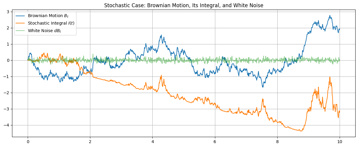
Here’s what things look like if we set $b(t) = \sin(t)$ and compare that vs $B_t$ as above. We’ll integrate both, and look at both “derivatives”:

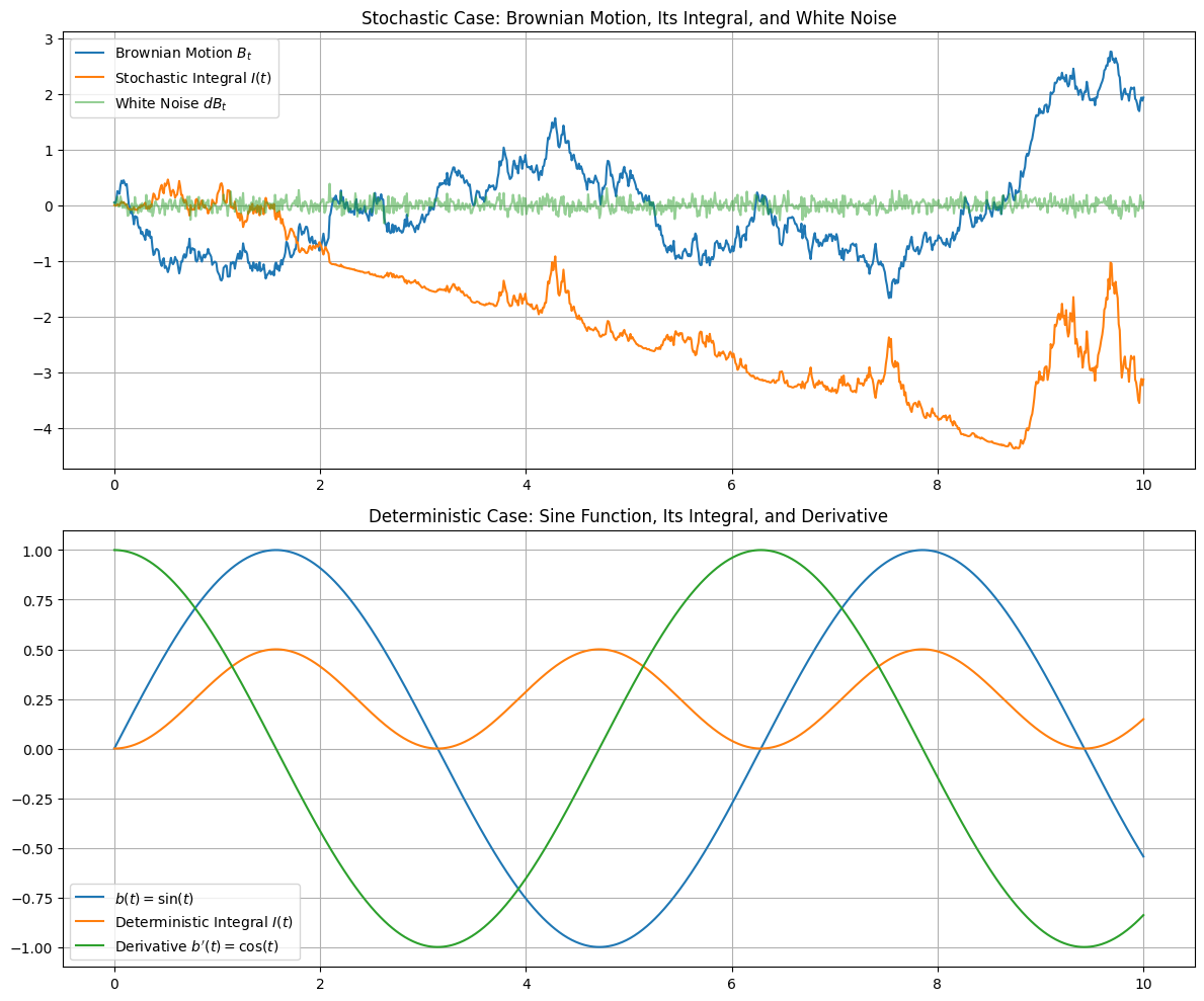
See what’s going on here? The “derivative” of $B_t$ is this super jagged ${\color{green}\text{green}}$ line. This line is so noisy that it’s samples are discontinous everywhere, and (as we’ll see later), it’s even unbounded on any interval. The only reason it “looks” bounded above is that we discretized it. (Another L for discretization.) No wonder that $\sum (B_{t_i} - B_{t_{i-1}})^2$ doesn’t vanish as the mesh size goes to zero.

On the other hand, the derivative of $b(t)$, namely $\cos(t)$, is smooth. The sum $\sum (b(t_i) - b(t_{i-1}))^2$ is approximately $\sum (t_i - t_{i-1})^2\cos(t_{i-1})^2 \leq \sum (t_i - t_{i-1})^2 \to 0$ as the mesh size goes to zero.

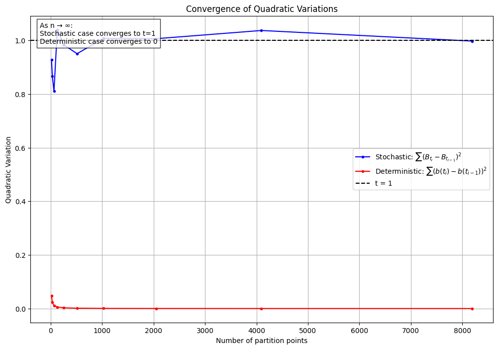
Just to beat this horse to death, let’s compare the sums $\sum (B_{t_i} - B_{t_{i-1}})^2$ vs $\sum (b(t_i) - b(t_{i-1}))^2.$ over $[0,1]$ through numerical calculation. From our arithmetic above, we know that $\sum (B_{t_i} - B_{t_{i-1}})^2$ should converge to $1$ and $\sum (b(t_i) - b(t_{i-1}))^2$ should converge to $0$ as the mesh size goes to zero. And in fact, here’s what things look like as the number of sub-intervals (x-axis) increases:

Our specific example with $\int B_s dB_s$ is an instance of Itô’s formula, the stochastic calculus analog of the Fundamental Theorem of Calculus. In the simplest case, if $f$ is a function with continuous second derivative, then Itô tells us that:

$$f(t) = f(0) + \int_0^t f^\prime(B_s)dB_s + \frac{1}{2}\int_0^t f^{\prime\prime}(s)ds.$$

The proof comes from the Taylor series for $f$. Write

$$f(B_{t_i}) - f(B_{t_{i-1}}) = f^\prime(B_{t_{i-1}})(B_{t_i} - B_{t_{i-1}}) + \frac{1}{2}f^{\prime\prime}(B_{t_{i-1}})(B_{t_i} - B_{t_{i-1}})^2 + h(B_{t_{i-1}}, B_{t_i})(B_{t_i} - B_{t_{i-1}})^2$$

Where $h$ is uniformly continous, bounded, and $h(x,x) = 0 \space\forall x$. For brevity, we’ll write $\Delta_{B_{t_i}} = B_{t_i} - B_{t_{i-1}}$.

$$f(B_{t_i}) - f(B_{t_{i-1}}) = f^\prime(B_{t_{i-1}})\Delta_{B_{t_i}} + \frac{1}{2}f^{\prime\prime}(B_{t_{i-1}})\Delta_{B_{t_i}}^2 + h(B_{t_{i-1}}, B_{t_i})\Delta_{B_{t_i}}^2$$

and when we sum things up

$$f(B_t) - f(B_0) = \sum_{i=1}^n f(B_{t_i}) - f(B_{t_{i-1}}) = \sum_{i=1}^n f^\prime(B_{t_{i-1}})\Delta_{B_{t_i}} + \frac{1}{2}\sum_{i=1}^n f^{\prime\prime}(B_{t_{i-1}})\Delta_{B_{t_i}}^2 + \sum_{i=1}^n h(B_{t_{i-1}}, B_{t_i})\Delta_{B_{t_i}}^2.$$

Following Chapter 8 of Steele’s Stochastic Calculus, we’ll write

$$A_n = \sum_{i=1}^n f^\prime(B_{t_{i-1}})\Delta_{B_{t_i}}, \quad B_n = \sum_{i=1}^n \frac{1}{2}f^{\prime\prime}(B_{t_{i-1}})\Delta_{B_{t_i}}^2, \quad C_n = \sum_{i=1}^n h(B_{t_{i-1}}, B_{t_i})\Delta_{B_{t_i}}^2.$$

I’m not going to work it through, but $A_n \to \int_0^t f^\prime(B_s)dB_s$, $B_n \to \frac{1}{2}\int_0^t f^{\prime\prime}(s)ds$, and $C_n \to 0$ in probability. Again, if $B_t$ (Brownian motion, not the sum $B_n$above) were replaced with a differentiable function $b(t)$, then $B_n \to 0$ and we’d recover the Fundamental Theorem of Calculus.

Trying to build more intuition for what’s different in the stochastic case, let’s go back to a sample plot from earlier:

The green line is an approximate/discretized version of $dB_t$. In code, we’re getting this by writing

dt = 0.001
dB_t = np.random.normal(0, np.sqrt(dt))

In some sense, $dB_t$ is the “derivative” of $B_t$. By definition $B_t = \int_0^t dB_s$. But what is $dB_t$? Earlier, we just used it as a shorthand for an integral equation. But is there a more direct way to think about it?

Yes

Do you remember the Dirac delta function? It’s a “function” $\delta_x(t)$ such that

$$I_x(t) = \int_{-\infty}^t \delta_x(s) ds$$

is $0$ if $t < x$ and $1$ if $t \geq x$. The delta function isn’t a function in the classical sense. There’s no function $\delta_x(t)$ with the desired property. But clearly $I_x(t)$ is well-defined, and in some sense $\delta_x(t)$ is its “derivative”. We might suggestively write $dI_x(t) = \delta_x(t)dt$.

It’s in this sense that we look for a “white noise” process $W_t$ such that $dB_t = W_tdt$. And we already know that $W_t$ should be infinitesimal Gaussian noise. Indeed, fixing a partition $\pi_n$ of $[0,t]$,

$$B_t - B_0 = \sum_i \frac{B_{t_i} - B_{t_{i-1}}}{t_i - t_{i-1}} (t_i - t_{i-1}).$$

Letting the mesh size go to zero, we want to define

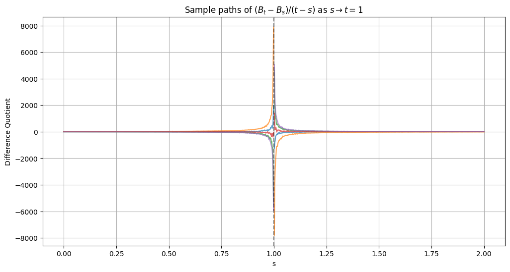
$$W_t = \lim_{s \to t} \frac{B_s - B_{s}}{s-t}.$$

As with Dirac, this limit doesn’t exist in the classic sense. Here are some sample paths for the limit, with $t = 1$:

We can do something similar to what we did with Dirac, though. We’ll basically just define $W_t$ as the “generalized process” for which

$$B_t = \int_0^t W_s ds.$$

It’s instructive to look at what this looks like for different resolutions. Here’s $W_t$ and the resulting $B_t$ for discretizations $dt = 0.1$, $dt = 0.01$, and $dt = 0.001$:

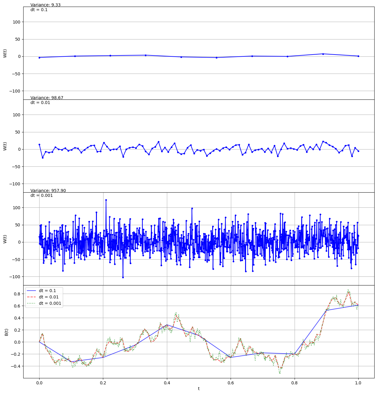
As $dt$ gets finer, $B_t$ becomes more “jagged”, which is what we want. To do accomplish this, the variance for $W_t$ has to explode. In fact, $W_t$ is pretty chaotic in general. The samples for $W_t$ are discontinuous everywhere, and they’re unbounded on every interval. For all these reasons, it’s hard to define $W_t$ as a “classic” process. Is there any alternative?

You may know that you can more formally define the Dirac delta as a “generalized function”. The idea is that a generalized function $f$ defines a linear functional from some space of functions $\phi$ to the base field $\mathbb{C}$ by

$$\phi \mapsto \int_{\mathbb{R}} \phi(x)f(x)dx.$$

Someone, probably Elias Stein, once explained this Biblically by saying “by their deeds ye shall know them”. The point is that if you know what $f$ does to every $\phi$, you know what $f$ is.

For the Dirac delta $\delta_x$,

$$\phi \mapsto \phi(x).$$

This is a well-defined functional that uniquely specifies $\delta_x$. What more is there to know?

And you can do an entirely similar thing for $W_t$. Define $W_t$ as the functional on a space of (square-integrable) stochastic processes $H_t$ by

$$H_t \mapsto \int_0^t H_s W_s ds = \int_0^t H_s dB_s.$$

This is a well-defined functional that uniquely specifies $W_t$. What more is there to know?